
Today we will use R astsa (Applied Statistical Time Series Analysis) library to analyze data and predict it with ARIMA model.
Load the data
|
1 2 3 4 5 6 7 8 9 10 11 12 13 14 |
library(curl) library(quantmod) library(rusquant) library(xts) library(utils) # ASTSA lib is for ARIMA library(astsa) # Load the data price.ohlc <- getSymbols("SBER", from = Sys.Date()-1, to = Sys.Date(), src = "Finam", period = "1min", auto.assign = FALSE) price.cl <- Cl(price.ohlc) # Display close price on plot plot(price.cl) |
Look at ACF and PACF
Compare auto correlation and partial autocorrelation functions for diff data
|
1 |
asf2(na.omit(diff(price.cl)) |
Output:
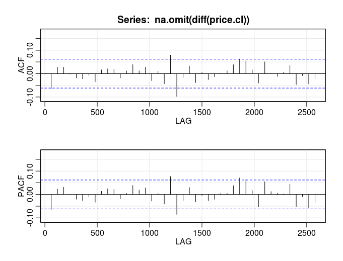
The ACF spikes are inside boundaries, it shows low auto correlation. Maybe ARIMA will not be a perfect model for that. Let’s look at first lags on PACF – only lag 1 spike is relatively big, so will use order 1 for ar (1,0,0) or ma (0,0,1).
Forecast
We need to choose (p,d,q) orders, where:
p – AR order
d– difference order
q – MA order
Let’s try Auto Regression model. PACF already showed us that only order 1 coefficients matter, so p = 1. We analyzing diff data, so d = 1. We don’t worry about MA in this example, so q = 0. Our (p,d,q) will be (1,1,0).
R code will be:
|
1 |
sarima.for(price.cl, n.ahead=100, 1,1,0) |
Output:
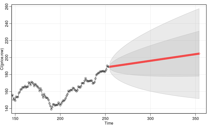
Where:
Black – original data
Red – prediction
Dark gray – 1 RMS prediction or 68% percentile
Light gray – 2 RMS prediction or 95 percentile.
Looks like a very broad prediction, so we need to try another model.
